29
68
Spécial « Congrès Acoustics 2012 »
Un nouveau procédé d’optimisation de la distance géométrique dans un système de reconnaissance automatique de chants d’oiseaux
Running the two methods side by side, both returned the
same result (a distance of zero) for perfect matches, but
the GD proved much more effective and robust for the
identification from similar (as opposed to exact) matches
to the reference.. The GD is computationally more expen-
sive than the Euclidean Distance but the advantages were
soon obvious.
Calls can by analysed at a rate as high as 100,000 per
second per processor but more typically the rate is 2,000
-3,000 per second, when a large number of different
reference templates are used simultaneously. The rate
depends on the call settings and the number of reference
calls in a reference template, with the rate increasing for
larger templates. A template is a file that is a mathemati-
cal image representing a collection of WAV file examples
of the call. Essentially a template contains the informa-
tion to build the images in Figures 1 and 2, for a collec-
tion of WAV reference files.
The Geometric Distance Concept
The most common measure of similarity is the Euclidean
Distance and as the name implies it uses the linear distance
between two patterns as a measure of the difference. The
Geometric Distance is measured as the angle between
two vectors that are the result of transforms on the origi-
nal data. For our purposes the GD is measured in degrees
with 90 degrees being the distance between two totally
dissimilar images. Differences of 3 to 3.5 degrees in CD
quality sounds are found between different sounds (as
subjectively judged by a human listener). In real world
soundscapes sounds that are similar are typically within
a GD of 5-6 or less of each other.
Dimensionality
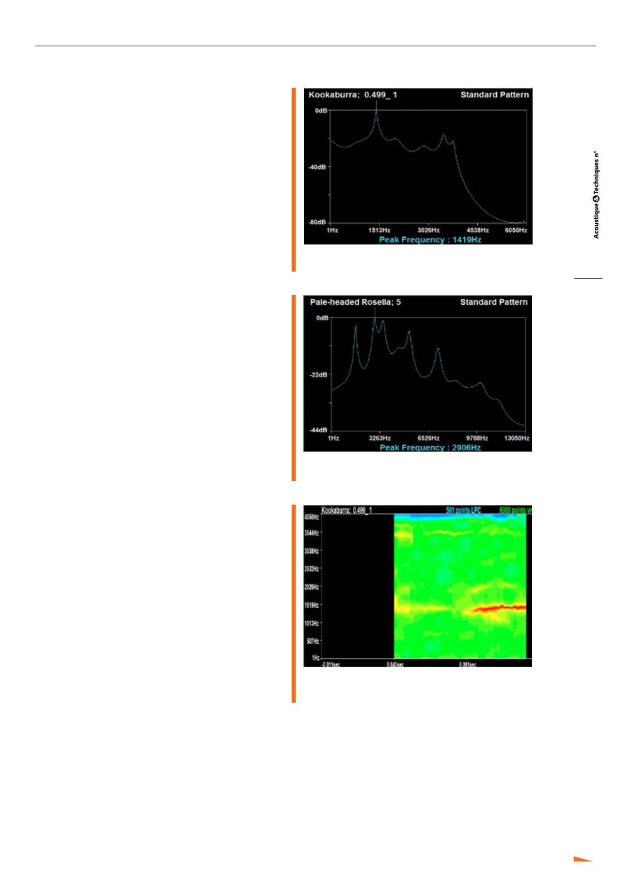
Most of the early work that we did used a 2-dimensional
image (see the example below of two different Australian
bird species in Figure 1: a Kookaburra call in Figure 1A
compared to a Pale-headed Rosella call in Figure 1B). It is
easy to see that the images are rather different and it is
these transformed images of the call that we compare.
To derive these images, the Linear Predictive Coding (LPC)
transform is used to calculate the frequency vs amplitude
spectrum of a frame typically of 2001 data points. This
was found to work well for most sounds, but it inherently
loses temporal information which is sometimes important.
The GD concept is N-dimensional (See Jinnai et al [7]) and
so it is possible to employ it on the more conventional
3-dimensional spectrogram (see the 3-D image below in
Figure 3), again calculated using the LPC. The 2-dimen-
sional GD process was found to be a lot faster than the
3-D and so we use both, choosing the 3-D only where it
is needed. It is also easier to visualise how the pattern
matching can be done using the 2-dimensional LPC than
with higher dimensional ones.
The Spectrum Transform
Initially the Fast Fourier Transform (FFT) was used as the
default transform and while some success was had with
it, we became concerned that the artifacts of the trans-
form were making the matching process less exact. By
running a lot of tests against the LPC using the same data,
we concluded that the LPC transform, though significantly
slower computationally than the FFT, was a more appro-
priate transform for our purposes.
Fig. 1A : The 2-D image of a Kookaburra call
Une image en 2-D d’un chant de Kookaburra
Fig. 1B : The 2-D image of a Rosella call
Une image en 2-D d’un chant de Rosella
Fig. 2 : The 3-D image of the same Kookaburra call as in Figure 1A
Une image en 3-D du même chant de Kookaburra que
pour la figure 1A
The LPC, first mooted in 1966 by S. Saito and F. Itakura of
NTT Japan, is widely used as a telecommunications speech
compression transform. Its use as a spectral transform
gives results that are largely consistent with the FFT but
with fewer artifacts. It can also be used to resolve small
signal fragments without the same loss of spectral resolu-
tion that is characteristic of the FFT. It is of course subject
to the limitations of the uncertainty principle and, as imple-
mented by us, does produce some artifacts.


