Version HTML de base


Journée SFA / Renault / SNCF
7
Acoustique
&
Techniques n° 44
€
Q
r
' 2
of the source at 1 000 Hz (autospectrum), the volume
velocity source being positioned at the driver’s ear
position.
SPL Calculation at Ear Receiver Points
The Sound Pressure Level resulting from the contributions
of the m sub-areas is given by equation 3 :
€
p
r
2
=
H
j
,
r
2
Q
eq
2
j
=
1
m
∑
j
( )
(3)
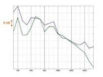
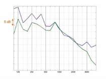
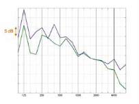
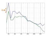
As we can see on figures 6 and 7, the correlation between
the simulation (or better said the recomposition
obtained with equation 3 and the experiments is quite
satisfactory for a full vehicle model, the level being
predicted within 3 dB(A) on the third octave spectrums
between 500 Hz and 3 150 Hz and below 2 dB(A) on the
overall Sound Pressure Level calculated between 500 Hz
and 5 000 Hz for both positions in the interior cavity and
for both road conditions.
We begin to observe discrepancies upper than 4 kHz due
to what has been identified by the probes manufacturer
as a «string resonance» of the hot wires of the
u
channel,
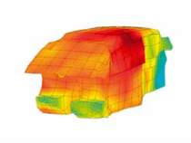
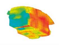
Fig. 5 : Transfer function 3DF map at 1 000 Hz, driver’s position
Fig.6 : SPL[dB(A)] recomposition VASM versus measurement, 4th gear 100km/h
Fig. 7 : SPL[dB(A)] recomposition VASM versus measurement, 2nd gear 100km/h
Vehicle Acoustic Synthesis Method 2nd Generation: an effective hybrid simulation tool to implement acoustic lightweight strategies