Version HTML de base


46
The finite element model of lumbar spine
Two models have been developed: one considers a single
motion segment (L4/L5) and one considers the lumbar
region of the spine (L1/L5), composed of four motion
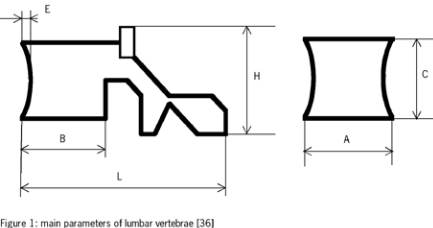
segments. A parametric finite element model of the lumbar
spine (L1-L5) and the motion segment (L4/L5) were gener-
ated in a CAD (Pro-Engineer) software application by consid-
ering the parametric equations describing the shape of
vertebra and intervertebral disc, as established by Lavaste
et al, (1992) [36]. The morphometric dimensions have
been considered as measured on various vertebral bodies
by Berry et al, (1987) [37]. Figure 1 illustrates the main
parameters of lumbar vertebrae. The rachis is composed
of 33 bodies (annulus, nucleus, endplate, cortical shell and
cancellous bone) and 54 zones of contacts are defined
between the bodies. The volumes in each of the models
were meshed separately with their meshing parameters.
Owing to the geometrical complexity of the spine, the
finite element mesh has to be fairly precise. The cortical
shell, the posterior elements, the cancellous bone and the
endplates were meshed by using 3D tetrahedral elements
with 10 nodes (Ansys software: Solid 187). This type of
element was selected because it allows a good interpola-
tion of external geometry. The nonhomogeneous structure
of the intervertebral disc was taken into account as it is
usually done in other finite element models. The annulus
fibrosus was modelized as a composite material.
Fig. 1 : Main parameters of lumber vertebrae [36]
The nucleus pulposus was modelled by using volumic
elements with a Poisson coefficient of 0.499 representing
quasi isovolomique behaviour. In this model, two types of
nonlinearity are considered, the geometrical nonlinearity of
the vertebrae and the nonlinearity of the contact between
the posterior elements. The contacts are modelled with
contact elements (Target 170 with 8-node, and Conta, 174
with 8-node). In vivo, a relative motion between posterior
elements is assured by articular cartilage. Consequently,
a very low coefficient of friction has been applied to model
the relative motion of cartilaginous structures. The contact
element used for modelling the connection between the
posterior elements has been chosen as ‘frictionless’ type.
Springs of low stiffness are added to the contact elements
model in order to insure continuity. The total number of
elements is about 36500 with 83808 nodes.
Authors
Test specifications
Specimen
number
Loads
N-Cycles
Observations
Gallagher [12]
Compressive and shear
loads
Frequency 0,33 Hz
36
25% to 60%
the ultimate
compressive load
1 000- 10 000
endplate fractures,
vertebral body fractures,
zygapophysial joint
disruption
Brinckmann [13]
Compressive
loadtriangular
Frequency 0,25Hz
Average age :
60 years
70
10- 80 %
the ultimate
compressive load
Max 5 000
endplate fractures,
vertebral body fractures
Hansson [14]
Compressive load,
sinusoidal
Frequency
: 0,5Hz
Average age :
60 years
17
60 to 100%
the ultimate
compressive load
1- 1 000
endplate fractures,
vertebral body fractures
Hardy [26]
Compressive load
sinusoidal
Frequency 2Hz
5
0,5 – 4,5 KN
10% to 84%
the ultimate
compressive load
200 to
1 290 000
endplate fractures,
vertebral body fractures
Adams [27]
Compression - flexion
:
sinusoidal
Frequency 0,76Hz
Angle 14°
Average age 35 years
52
3500 N
65% the ultimate
compressive load
14 400
(average)
Slipped disk (21%
)
&
endplate fractures,
vertebral body fractures
Liu [28]
Compressive load
sinusoidal
Frequency 0,5Hz
Average age 50 years
11
37 à 80%
the ultimate
compressive load
2 000
50%
: endplate fractures,
vertebral body fractures
for 60%.
Lafferty [29]
Flexion. Compression
2Hz
17
142 -979N
20% to 70%
the ultimate
compressive load
26 to 196 000
apophyses fracture
Table 1 : Synthesis of fatigue tests