Version HTML de base


“Uncertainty-noise” Le Mans
29
Acoustique
&
Techniques n° 40
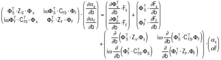
The sensitivities of the modal coordinates are obtained by
solving the complex-valued system of equations:
Note the close similarity between these relations and the
sensitivity analysis in physical coordinates. Once the system
is projected in the modal basis, the sensitivity analysis can be
performed using similar solution sequences, which can lead to
a substantial profit in an algorithmic implementation.
An alternative to solving the above equation for the sensitivities
of the modal coordinates is to performMonte-Carlo simulation
on the equation giving the modal coordinates [12]. In fact, this
discrete system is of reduced size due to themodal formulation
and repeated solutions are not anymore computationally-
intensive with regard to the initial eigenproblem solution.
Moreover, using Monte-Carlo simulation enables to handle the
nonlinearity between the modal coordinates and the random
design parameters without any restriction on the variability
level (which is especially useful at resonances).
Random field modeling
The concept of random field [13] is often resorted to as a
mean to model the spatial variability of the material parameters
(sometimes improperly considering the lack of experimental
knowledge in the uncertain spatial behaviour of material
properties). As a consequence of its continuous character,
the random field requires an appropriate discretisation, leading
to the identification of a finite set of random variables. This
set has to satisfy two opposite requirements: on the one
hand, it should represent accurately the original continuous
random field and, on the other hand, it should involve the
smallest number of random variables since the computational
cost of response variability analysis grows significantly with
this number. For instance, the spectral SFEM, based on
the Karhunen-Loeve expansion of the random field, uses
polynomial chaoses on which the stochastic response is
projected [9,11].
The identification of this projection requires the solution of an
algebraic system of order P x N, where N is the size of the
deterministic problem and P is the number of terms (basic
random polynomials) involved in the projection. This number
P grows prohibitively as soon as the global order of the
method and/or the number of discrete random variables are
increased. The Monte-Carlo simulation method is known to
provide the best variability estimations as soon as the number
of samples involved in the analysis is sufficient. Whereas it
is difficult to estimate this number, it should be increased
with the number of random variables involved in the model,
which results in a substantial increase of the computational
time. Finally, the perturbation method, based on a low-order
response representation, estimates the response variability at
a relatively low additional cost with respect to the deterministic
analysis, which is however proportional to the number of
random variables in the stochastic analysis.
Reduction techniques of the finite set of random variables are
however available [2]. The first well-known reduction technique
relies on the finite element mesh to perform the discretization
of the random field. A midpoint technique enables the
identification of a set of correlated random variables from the
covariance function of the random field, each variable being
related to a particular element. A decorrelation procedure
based on the spectral analysis of the discrete covariance
matrix is performed in order to identify a reduced number of
stochastic basic components. As an alternative to the midpoint
discretization, a (numerical) Karhunen-Loeve decomposition
is possible, the truncation of which allows to extract the
stochastic components that introduce the major variability
in the model.
The criteria leading to the definition of the random field
discretization and analysis meshes are different, the first being
related to the correlation length of the random field, the second
being related to the stress gradients or the wave speeds in
the model. Generally, the second criteria is more demanding
than the first one. It results from this observation that using
the finite element mesh for the random field discretization can
lead to increase computational costs and even to numerical
inaccuracies. A second reduction technique is thus possible
in which a different discretization mesh is used.
In contrast with random variable models, the random field
model enables the development of a compensation effect, i.e.
a reduction of the response variability due to the correlation
structure of the random field. Fig. 1 illustrates, for the simple
configuration of a clamped-free beam with random flexibility F
(analytical solution is available [2]), the close relation between
the compensation effect and the filtering of the stochastic
components of the random field by the dynamic system.
First, the intensity of the compensation effect is related
to the correlation structure of the random field. A more
important compensation effect is observed in the case of a
low correlation length.
The error that would be obtained if the correlation properties
of the field was wrongly taken into account would thus be
notable. Second, the compensation effect strongly depends
(8)