Version HTML de base


“Uncertainty-noise” Le Mans
27
Acoustique
&
Techniques n° 40
on a two-phase model (Biot model for instance) involving a
substantial number of parameters not easy to measure and
quite frequency dependent …
In this context, the steady development of computational
mechanics over the past five decades, supported by
continuously more efficient computing tools, gives the
opportunity to define structural models reaching a relatively
high level of refinement. These models however require
the definition of many material properties, geometrical
parameters, load conditions, ..., the exact knowledge of which
could not be possible. Some compromise has therefore to
be found.
In a vibro-acoustic context, the general modeling strategy
should take into account the fact that uncertainties are usually
higher for the (structural) dynamic component than for the
acoustic component. This is due to the relative simplicity
of the acoustic propagation operator with respect to the
elastodynamic operator. In most of the cases, the quality
of acoustic predictions strongly depends on appropriate
boundary conditions (especially velocity or acceleration
constraints).
An important source of uncertainty is attached to boundary
conditions (in general) and, particularly, to loading or
kinematic excitations of the model. Here, uncertainties occur
simultaneously on the mathematical model stage (nature of
the excitation, spatial distribution, spectral content or time
histories, …), on the numerical model stage (discretization of
the selected excitations, sampling procedures, …) and on the
parameter definition stage (intensities, probability distributions
of the loads, stationarity or unstationarity of the random
processes…). Methods for handling uncertainties in the load
conditions of dynamic models are now well established.
The related semi-empirical spectral models for usual random
distributed loading (diffuse field, turbulent boundary layer) are
important components of vibro-acoustic simulations. This is, at
least partially, due to the difficulty to simulate highly turbulent
unstationary flows with traditional CFD tools at high Reynolds
number.
The uncertainty sources described above are also hard
to quantify independently. More precisely, it is difficult to
determine the uncertainty level implied in the modeling
stage, that is involved during the mathematical modeling
process and its numerical implementation. Practically, there
are no other means than to consider that these uncertainty
sources are negligible or are covered by the variability of
the model parameters. This last assumption, although it has
no physical foundation, seems to be generally accepted in
the literature. Recently Soize [4] developed non-parametric
approaches in order to handle these uncertainties in a more
rational way. This model has been extended recently to vibro-
acoustic studies [5].
Based on the above observations, one is forced to admit
that a given amount of uncertainty or irreducible variability is
present in each vibro-acoustic model, and that simply carrying
out a deterministic analysis leads to an error, which should
be at least estimated. Non-deterministic approaches are
thus a natural and necessary extension of present analysis
techniques.
Mechanical and geometric uncertainties
Stochastic Finite Elements
Amongst all numerical procedures in non-deterministic
computational mechanics, the stochastic finite element
method (SFEM) [6,7] has been developed and applied to
the reliability and response variability assessment of static
and dynamic, linear and non-linear problems. In the context
of second moment approaches for the response variability
assessment, the perturbation SFEM [8], the spectral SFEM [9]
and the Monte-Carlo simulation method are available.
The selection of a particular method often relies on
considerations about computational requirements with
regard to the dimension of the problem (number of degrees
of freedom (dofs) and number of uncertain parameters) and
to the considered variability level. The Monte-Carlo simulation,
from its general formulation, is able to cope with high variability
levels but suffers from prohibitive computational costs.
Recent developments have thus been aimed at optimizing
its application by using variance reduction techniques or by
resorting to parallel computing [10]. In the spectral SFEM, the
number of involved random variables is very critical so that
appropriate algebraic solvers, based on the particular structure
of the problem, have been developed [11]. The perturbation
method has been widely applied to stochastic problems since
it usually requires low computational resources. It however
suffers from the fact that it relies on a low-degree polynomial
approximation of the structural response and is thus aimed
at solving models involving a low variability level of the design
parameters [2,12].
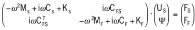
Considering a linear vibro-acoustic problem stated in the
frequency domain, the discretization using conventional finite
elements leads to the following complex-valued algebraic
system:
(1)
where
ω
is the circular frequency;
U
S
is the vector of nodal
displacements of the structure;
Ψ
is the vector of nodal
potentials of the fluid;
F
I
is the excitation vector,
M
I
, C
I
and
K
I
are the mass, damping and stiffness matrices for the
fluid (I=F) or the structure (I=S) and
C
FS
is the fluid-structure
coupling matrix. Defining a set of random variables (either
of material or geometrical nature) b
i
(
θ
) (i=1, …, q), each of
the above vectors and matrices is a random quantity and
implicitly exhibits a
θ
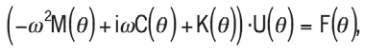
-dependence. Note that this systemmay
be rewritten in a canonic form for dynamical systems:
(2)
where
U
(
θ
) is the vector of both potentials or displacements,
F
(
θ
) is the excitation vector,
M
(
θ
) is the system mass matrix,
C
(
θ
) is the system damping matrix and
K
(
θ
) is the system
stiffness matrix.